Determinants of Crime in Brazilian Southeast: Applications of Spatial Econometrics Techniques
Overview
The intentions of this post are to present the main aspects of my final thesis, including the objectives, theoretical framework, literature review, methodology, and results. The full version is available in Portuguese. The content was adapted to a portfolio post structure, emphasizing the key points and bringing out the main results.
Abstract
LUCAS, João Pedro Toledo Tricoli. DETERMINANTS OF CRIME IN BRAZILIAN SOUTHEAST: APPLICATION OF SPATIAL ECONOMETRIC TECHNIQUES. 2023. Undergraduate Thesis. School of Economics, Center for Economics and Business, Pontifical Catholic University of Campinas, Campinas, 2023.
Several fields of knowledge delve into the determinants of criminality, aiming to understand “how” and “why” individuals commit crimes. This study seeks to analyze the determinants of crime in the southeastern region of Brazil by means of spatial econometric techniques based on the theoretical framework of crime economics and Exploratory Spatial Data Analysis (ESDA). The Spatial Lag (SAR) model was applied to the homicide rate (per 100,000 people) in 2010, smoothed by empirical Bayesian methodology, at the municipal level and across socio-economic variable groups encompassing inequality, predisposition of young men, family instability, education, urbanization, and risk. Including the spatial component does not validate the significance found in the simple linear model for variables such as inequality and young men’s predisposition to crime. Conversely, it highlights the positive impact of education, family stability, urbanization, the unemployment rate, and apprehension risk in metropolitan regions. It is worth noting the presence of high crime clusters in Rio de Janeiro and Espírito Santo and low crime clusters in the regions of Minas Gerais and São Paulo. In summary, policies aimed at reducing inequalities, promoting education, strengthening family stability, investing in security, and creating job opportunities have the potential to have positive impacts on reducing homicide rates.
Keywords: Economics of Crime; Spatial Econometrics; Spatial Exploratory Data Analysis; Brazilian Southeast.
Introduction
Many fields of science search for answers about criminality; the most famous is sociology, with empirical studies, philosophy, and other areas. The main question in the scope of criminology is “how” and “why” people commit crimes.
The economic contribution comes from Gary Becker, an economist from the University of Chicago. In the study Crime and Punishment: An Economic Approach, Becker used a mathematical framework where, assuming rationality, a person would commit an illegal act when considering that the utility of committing such an offense outweighs the utility he could have by using his time in another legal activity.
The utilitarian vision brings an ideal to the choice of a rational individual, weighing the risks and possible rewards when choosing a criminal practice. The inclusion of socioeconomic variables in mathematical modeling aims to identify the possible determinants that influence the individual’s decision.
Therefore, this work aims to study the economy of crime with a theoretical framework based on Becker’s theory (1968), using spatial econometrics modeling and Exploratory Spatial Data Analysis (ESDA) to identify the relationship between the main socioeconomic variables and crime in the southeast region of Brazil.
Fundamentals of the Crime Economy
The main consideration of Becker’s model is based on the individual’s decision, considering the cost-benefit of allocating their time to a legal or illegal activity.
\[b>cp\]
Where \(b\) is the benefit to the individual for practicing an illegal act, \(c\) is the cost of the criminal activities, and \(p\) is the probability of apprehension.
With that, the individual is encouraged to choose criminal activity when the benefit \(b\) exceeds the cost of criminal activity \(c\) multiplied by the chance of being apprehended \(p\).
Becker divides the analysis into four main topics that cover mathematical modeling. The first is damage, which is the difference between the gains to the criminal individual and the cost caused to society by the illegal activity. It fallows with the cost of apprehension and conviction, bringing the idea that increasing the probability of a felony being convicted would increase the cost for the criminal in practicing illegal activities.
The last two are offenses and punishments. Overall, it is said that increasing the probability of discovering the crime, along with the probability of being condemned and the punishment that it would receive, would impact the risk, changing the balance in the decision-making process of the criminal individual.
It is important to mention that the punishment should always fit the crime because a high increase in the risk could make minor felonies more violent because the risk is so great but other rewards in legal activities are still minors.
Literature Review - Determinants of Crime
The literature review looks at the main question surrounding similar studies in crime economy: “What are the socioeconomic variables that impact criminal activities?”. The studies looked for different countries and periods to compare the variables chosen and their main impact.
Overall, the literature presents a variety of variables, as well as their justifications in terms of cost and benefit, that are based on the individual’s rationality and interpretation of socioeconomic impacts.
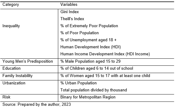
Therefore, it was possible to identify five main categories, namely, inequality, the predisposition of young men, education, family instability, urbanization, and risk. This division will be used as the basis for the methodological process for building and estimating the model.
Methodology
The present work aimed to apply spatial econometrics and Exploratory Spatial Data Analysis (AEDE) given the assumptions presented in Becker’s theory (1968). The contributions of similar studies visited in the literature review were taken into account, serving as a basis for structuring the model and selecting socioeconomic variables.
The methodology aims to discuss the fundamental analyses surrounding the concepts of Spatial Econometrics and Exploratory Analysis of Spatial Data (AEDE). The main topics visited were: Spatial Autocorrelation; Neighborhood Matrices; Moran Indicator and Regression Models, namely, Ordinary Least Squares Method (OLS); Spatial Lag Model (SAR) and Spatial Error Model (SEM), along with the process of choosing spatial regression by Anselin. L (2005).
Results
The study starts with the construction of a model based on the main variables chosen as the determinants of crime. The dependent variable, homicide rate (100,000 people), was chosen. The variable passed to a Bayesian empirical smoothing process; the goal was to deal with high variance, especially in small municipalities. The methodology helps in making predictions or estimating values based on observed data. In simpler terms, it’s like using past information to make educated guesses about what might happen next.
<!DOCTYPE html><img src="/images/Figura_Not_Smooth_Homicide_Rate.png" alt="Figura_Smooth_Homicide_Rate" />
<img src="/images/Figura_Smooth_Homicide_Rate.png" alt="Figura_Smooth_Homicide_Rate" />One main problem in selecting the independent variables is that even after the creation of a category-based filter, there are still many variables that might explain the variability of the homicide rate. Because of that, a stepwise regression was built based on a selection of independent variables. In general terms, stepwise regression is a technique that starts with a complete model and, at each step, gradually eliminates independent variables from the regression model.
The final model provided the best fit, although manual alterations were needed to deal with multicollinearity. Mostly, two variables selected in the stepwise regression were removed, the HDI index and the income HDI index. The dependent variable was transformed to log, being chosen as the best fit in the stepwise regression. The final independent variables can be seen in Table 1 alongside the main category they fall into.
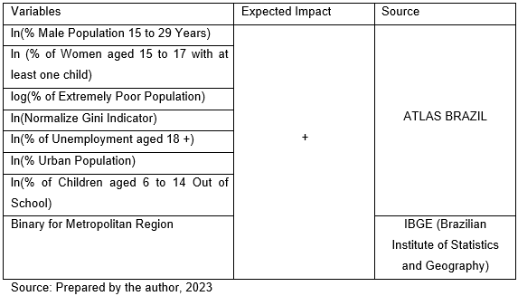
Frame 2 presents the main variables and the expected impact that they will have on the log-smoothed homicide rate (100 thousand people). The results of the OLS model are shown in Table 2.
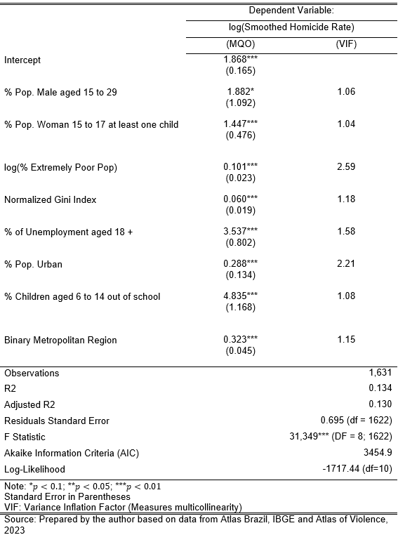
The model falls into the expected results, with all variables with the anticipated sign being statistically significant the same as the model, and the independent variables explain 13% of the variability of the dependent variable. The model also doesn’t present a problem with multicollinearity, with all variables having \(VIF < 2.60\).
The OLS model brings the first idea, and if it is possible to continue the investigation about spatial autocorrelation, In this way, the OLS uses squared errors as the basis for estimating the coefficients; however, the regression assumes that these residuals have constant variance (homoscedasticity). In the case of data with Spatial Autocorrelation, the errors may not be stochastic (random), thus existing patterns of association between nearby regions.
The main factor is that heteroscedasticity (residuals have unequal variance) violates the principle of OLS regression, being present in errors in spatial relationships and raising the hypothesis that the spatial component must be treated in a special way. As a result, regression using the OLS with data that have a spatial relationship is not recommended since the estimates may contain bias due to a violation of the principle of homoscedasticity of errors. Therefore, despite being a good start to exploring the relationships between variables, other options are recommended, the main ones being Spatial Lag (SAR) and Spatial Error (SEM).
Neighboring Matrix
The choice of the neighboring matrix is a key step in spatial regression because it is a mathematical way to express who is and who is not the neighbor for a given region. There are many ways to represent the neighboring matrix; in this study, the queen contiguity of order one was used. Exemplified by chess, we have that in the queen contiguity method, all adjacent polygons, including those found at the vertices, are considered neighbors. They are also given proportional weight to each neighbor; Figure 2 brings out the main idea.
Spatial Autocorrelation - Moran I and LISA
After the construction of the OLS model and the confirmation that the proposed relationship holds statistical significance while the impacts fall under the imposed hypotheses, the process begins to identify if there is any Spatial Autocorrelation.
Spatial Correlation refers to the strength of the association between cases and between space, explaining how similar observations are between neighbors. In this case, we could have, as an example, extremely violent regions that spread higher levels of violence to nearby regions. The intensity of violence in a region affects the intensity of violence in nearby locations. In short, Spatial Correlation brings force between variables in space.
The standard deviation of the residuals is used as a visualization method; it indicates how much the data differs from the mean. In this case, each standard deviation becomes a category in the choropleth map that can be visualized in Figure 3.
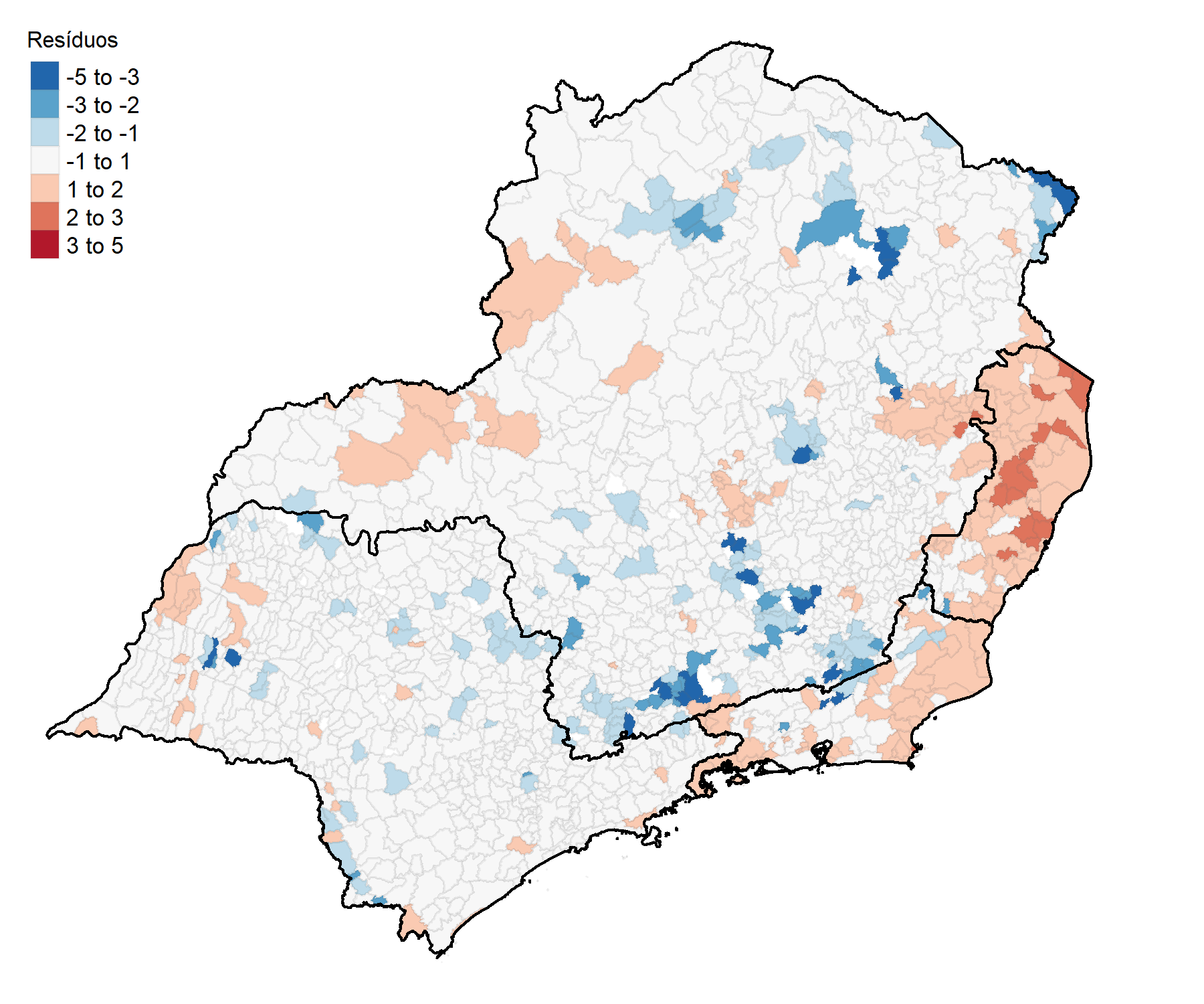
The result shows that certain areas in red are overestimating and other areas in blue are underestimating. Furthermore, it is possible to visualize clusters, mainly in the states of Rio de Janeiro and Espírito Santo, indicating that Spatial Autocorrelation possibly exists.
One of the possible steps to attest to spatial autocorrelation is the Moran I test, which provides the linear model and the neighborhood matrix, in this case the queen contiguity matrix with order one. The result can be seen in Table 3.
The Moran I bring a coefficient that quantifies the strength of the Spatial Correlation, being between 1 and -1. Thus, 1 would indicate the existence of a strong positive Spatial Autocorrelation, and -1 a negative one.
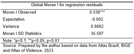
The test presents statistical significance, and the Observed Moran I indicate a moderate and positive autocorrelation. Therefore, we can conclude that for this model, the residuals are systematically related.
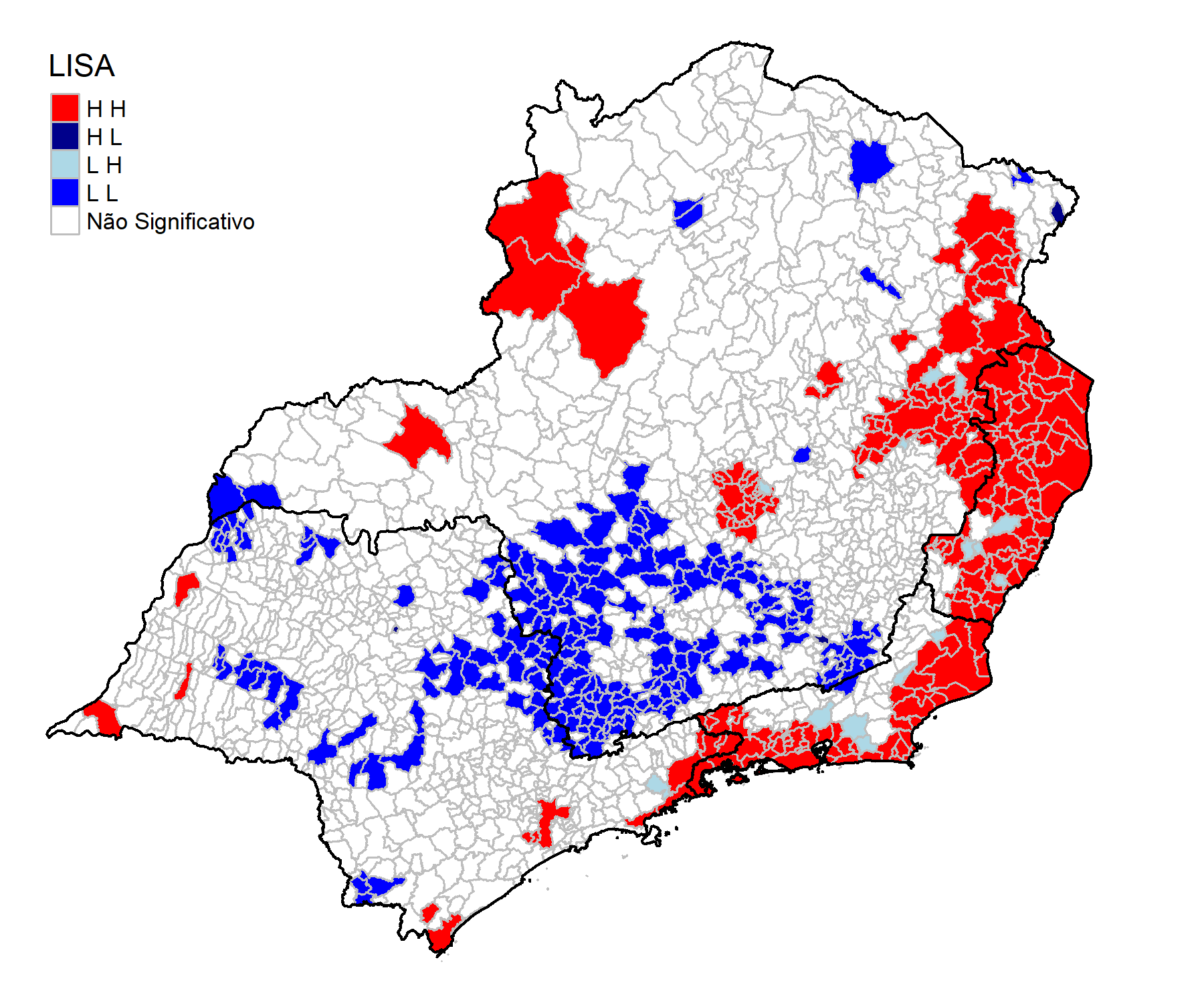
In order to analyze Spatial Autocorrelation, the Local Spatial Association Indicator can be used. It specifies in a local way, allowing you to find clusters of autocorrelation. The categories are High-High, Low-Low, High-Low and Low-High, meaning similarity. For example, the High-High category would show that high levels of violence in a given municipality are fallowed by a high level of criminality among its neighbors.
In general, it is possible to identify areas where the log-smoothed homicide rate (100 thousand people). presents high levels and is followed by their neighboring municipalities. The same interpretative logic follows for the other categories.
The representation Figure 4 shows the categories and specifies the clusters in regions where the Moran location test obtained statistical significance at a p-value < 0.1.
Choosing the Spatial Regression
With the Spatial Autocorrelation tested, the next step is to find the most suitable Spatial Model. There are two main models that can be used to represent Spatial patterns: the Spatial Lag (SAR) and Spatial Error (SEM).
The Spatial Lag (SAR) is similar to the OLS but adds a lagged version of the dependent variable as an independent variable. It is used for regression when the dependent variable is influenced by its neighbors, making it one of the most common ways to investigate spatial dependence.
\[y = \rho Wy + x\beta + u\]
Where the values of neighbors \(y\) that have the weight of the spatial matrix \(W\) are multiplied by \(\rho\), representing the autoregressive coefficient for the dependent variable. While \(\rho\) expresses the strength of the spatial autocorrelation presented in the dependent variable.
In this case, the estimate of \(y\) depends on \(x\beta\) and \(\rho W\); therefore, the interpretation of \(x \beta\) is not the same as in the OLS, as we consider the spatial effect for the variable \(y\) in the neighborhood matrix.
Therefore, when we want to discover a spatial interaction process and the effects of neighbors on the dependent variable, we can use the Spatial Lag (SAR) model.
On the other hand, it is also possible that the Spatial Error (SEM) could be a better fit for the Spatial pattern in hand. In sum, the Spatial Error model (SEM) is used in regression when we believe that the observed spatial autocorrelation is related to the spatial process whose intensity varies throughout space (Spatial heterogeneity).
This model deals with spatial heterogeneity by estimating the spatial coefficient within the regression error. The model includes an error term for neighbors, defined by the neighborhood matrix with weights \(W\), along with the usual error term.
\[y = x \beta + u\] \[u = \lambda Wu + \varepsilon |\lambda|\] \[u = u = \lambda Wu + \xi\]
An example would be the study of crime in an area that would be influenced not only by its factor but also by crime in neighboring regions. In this way, the model captures the spatial correlation through error terms.
The selection of the Spatial Regression falls under Anselin. L (2005) methodology. The process begins with the construction of an OLS model (OSL), with the objective of studying the relationship between the variables and highlighting the existence or not of Spatial Autocorrelation in the residues.
Furthermore, the OLS model provides the first diagnosis of the relationship between variables, being able to explain outliers and extreme multicollinearity.
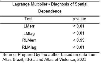
Anselin. L (2005) uses two Lagrange multiplier tests to access spatial dependence; however, it is common to access the residuals of the OLS model and perform the Moran I test. To identify Spatial Autocorrelation, it is necessary to create a neighborhood matrix. The choice of which type of matrix is based on the nature of the relationship studied.
With both Lagrange multiplier tests, we can identify the Spatial Autocorrelation of the model and, more specifically, select which one would provide a better fit: Spatial Lag (SAR) or Spatial Error (SEM). The results can be seen in Table 4. Both Lagrange multiplier tests were made, and the Spatial Lag (SAR) was chosen as the robust one.
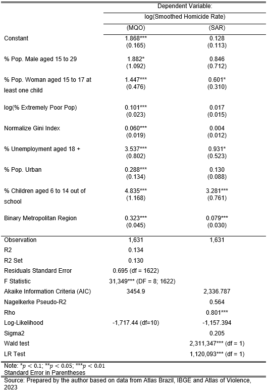
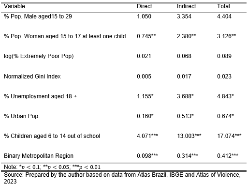
The final results can be seen in Table 5. The addition of the spatial component in the Spatial Lag (SAR) did not hold significance for variables such as % Pop. Male 15 to 29, log(Extremely Poor Pop), Normalized Gini Index, % Pop. Urban.
On the other hand, the Log-Likelihood and Akaike Information Criterion (AIC) measures show improvement when compared to the OLS model. The Log-Likelihood increases from -1,717.44 to -1,157.394, while the AIC reduces from 3454.9 to 2,336.787.
In summary, AIC is a statistical measure for model selection, balancing model adjustment, and complexity. Lower values of this indicator indicate better balance and adjustment. On the other hand, Log-Likelihood is a measure that represents how well the statistical model explains the observed data; higher values indicate a better fit of the data.
It is worth mentioning that the impact of the variables cannot be interpreted only on the predictor indicators because it is not possible to interpret the coefficients as marginal effects due to spatial dependence.
We have that the change of \(i_{th}\) predictor municipalities can affect the result of the \(j_{th}\) region. The two situations are the direct impact of a predictor observation on its own result and the indirect impact of a neighboring predictor observation on its result. Table 5 shows the impact results for the estimated model.
Discussion
The present work aimed to analyze the determinants of crime in southeastern Brazil, using Becker’s theoretical framework (1968) and a review of similar studies for the process of choosing variables for the determinants of crime. Econometric modeling and application of Exploratory Spatial Data Analysis (AEDE) tools and methodologies were used to create and estimate the models, observing the impact of the variables and considering the spatial component.
It was evident that for this analysis structure, considering cross-section data from the year 2010 at the municipal level for southeastern Brazil in both dependent and independent variables, the addition of the spatial component does not fully support the hypothesis explained in the OLS model. The interpretative results of Spatial Lag are shown in Table 6.
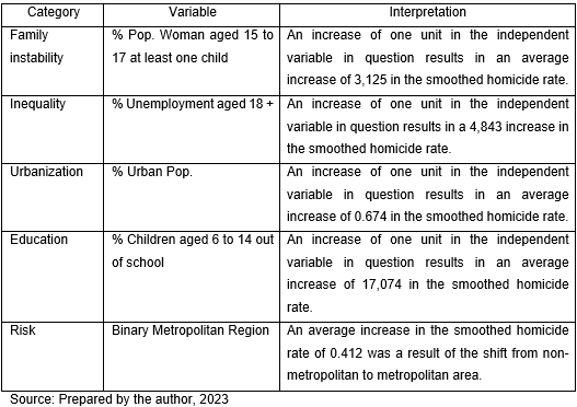
The model indicates that the most sensitive variable was the percentage of children aged 6 to 14 years out of school, indicating that an increase of one unit in the variable in question would have an average impact of 17,074 on the log-smoothed homicide rate (100 thousand people).
The idea follows the variables of unemployment percentage of people aged 18 or over and percentage of female population aged 15 to 17 with at least one child. Therefore, a one-unit increase in the independent variable in question impacts on average 4,834 and 3,125 on the log-smoothed homicide rate (100 thousand people), respectively.
These indicators alone bring an important cyclical idea, as they conclude that there is a high sensitivity of the young population to socioeconomic variables that affect this group. Education is easier to observe since it is directly linked to the young population; however, it has a direct and indirect impact on development as it leads to future unemployment and serves to minimize family instability, which in this analysis was done through young mothers with at least one son.
In the Brazilian case, it was concluded that unemployment has a positive impact on crime. The assumption converges with the theories studied, where low rewards for legal activities make illegal activities more attractive. Unlike education, employability tends to be more sensitive to government policies with immediate returns; however, it is worth thinking about where the root of the problem lies.
The established relationship provides an indicator that certain variables tend to work differently in urban centers, which is why the urbanization variable present in this study follows the results of the literature. A one-unit increase in the variable in question impacts, on average, 0.674 on the log-smoothed homicide rate (100 thousand people).
Reflection on the result follows the assumption that large urban centers have a structure more conducive to crime. It is possible to observe these differences in relation to impact variables, mainly in terms of inequality and risk. The problem of urban agglomeration is difficult to solve through government policies, with a greater focus on structural differences that lead large urban centers to become a more attractive environment for crime.
Therefore, one of the points related to urban centers, which are part of the structure that makes them more prone to crime, is risk. Increasing the risk of discovery, apprehension, and conviction tends to reduce crime, as it is directly related to the individual’s decision-making process.
The inclusion of the binary variable for municipalities belonging to metropolitan regions makes the assumption that large centers tend to have lower risk, as confirmed by the result, indicating that the change from a non-metropolitan region to a metropolitan region tends to have an average impact of 0.412 on the log-smoothed homicide rate (100 thousand people).
The risk has important relevance, as it alone may not have a positive impact on the reduction of crime and may create the opposite effect. An example would be to drastically increase the penalty for conviction for a minor crime; this could lead to a higher level of violence since the risk has increased drastically; however, the opportunity for legal activities is still extremely low, maintaining the balance of individual decisions and increasing data for society.
In general, Becker’s (1968) vision contributes to organizing and measuring the decision-making process, allowing strategies to be devised to mitigate the increase in crime. Therefore, it is plausible to identify important variables for the individual’s decision-making process in relation to criminal activities, bringing greater effectiveness to government actions and public security policies.